How to calculate the Betweenness Centrality against NebulaGraph

​Betweenness Centrality (BC for short) reflects the significance of vertices in the entire network. This article will introduce how to compute Betweenness Centrality against NebulaGraph.    

Relevant Concepts

Centrality represents how central a vertex is in the entire network graph, including Degree Centrality, Closeness Centrality, and Betweenness Centrality, etc. Degree Centrality reflects the popularity of a vertex by counting the number of its incoming and outgoing edges, while Closeness Centrality computes the sum of the length of the shortest paths between a vertex and all other vertices in the graph. Thus, the more central a vertex is, the closer it is to all other vertices.

Betweenness Centrality counts the number of times a vertex appears on the shortest path between any two other vertices, so as to represent the significance of this vertex to the network connectivity.

The Betweenness Centrality of a vertex is the proportion of the number of paths passing through this vertex in all the shortest paths to the total number of shortest paths.

Calculating the Betweenness Centrality of a vertex in a graph can be conducted in a weighted graph or in an unweighted graph. For unweighted graphs, Breadth-First Search (BFS for short) is used to find the shortest path, while for weighted graphs, Dijkstra’s algorithm is used.

The following algorithms are all targeted at undirected graphs.

Applicable Scenarios

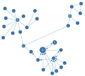
Betweenness Centrality reflects the significance of vertices in the entire network by measuring how a vertex bridges all other vertices in a graph or network. As we can see, Vertex C in the following figure acts as an important bridging vertex.

Betweenness Centrality can be used to identify

a. The intermediary entities in anti-fraud scenarios in the field of financial risk control.

b. Specific disease control genes in the medical field to improve drug targets.

Betweenness Centrality Algorithm

The Betweenness Centrality of a vertex can be computed as follows:

$$C_B = \sum_{s{\not=} v {\not=} t \in V} \frac{\sigma_{st}(v)}{\sigma_{st}}$$

（Formula 1）

In this formula,

$\sigma_{st}(v)$ is the number of shortest paths from Vertex s to Vertex t.

$\sigma_{st}$ is the number of shortest paths that pass through Vertex v.

Vertex s and Vertex t are a pair of vertices belonging to the vertex set.

To make it more convenient, the betweenness of each pair of vertices can be computed as:

$$\delta_{st}(v) = \frac{\sigma_{st}(v)}{\sigma_{st}}$$

（Formula 2）

So Formula 1 can be replaced by Formula 2, which gives rise to Formula 3 as follows:

$$C_B(v) = \sum_{s{\not=} v {\not=} t \in V} \delta_{st}(v)$$

（Formula 3）

Solution Procedure

To get the Betweenness Centrality of Vertex v, namely to get $$\frac{, we need to know whether Vertex v lies on the path from Vertex s to Vertex t.

(1) To know whether Vertex v lies on the shortest path from Vertex s to Vertex t, use the following formula $d_G$ represents the shortest path from Vertex s to Vertex t):

If Vertex v lies on the shortest path from Vertex s to Vertex t, then $$d_G(s,t) = d_G(s,v) + d_G(v,t)$$ is satisfied.

（Formula 4）

$d_G(s,v)$ and $d_G(v,t)$ are mutually independent. According to the rules of combination, the total number of shortest paths from Vertex s to Vertex t is the product of the number of shortest paths from Vertex s to Vertex t and the number of shortest paths from Vertex s to Vertex t.

Based on the above two situations, Formula 5 can be inferred:

$$\sigma_{st}(v) = \begin{cases} \sigma_{sv} \times \sigma_{vt} &\text{if } d(s,v) + d(v,t) = d(s,t) \ 0 &\text{if } other
\end{cases}$$

（Formula 5）

（2）According to the above formula, we can get the conclusion that the number of shortest paths from Vertex s to Vertex t that pass through Vertex w is the result of

$\sigma_{st}(w) = \sigma_{sw} \times \sigma_{wt}$. In the graph, Vertex v is the preceding vertex of Vertex w. Therefore, the formula to count the number of shortest paths from Vertex s to Vertex t passing through Vertex v to Vertex w is:

$\sigma_{st}(v,{v,w}) = \sigma_{sv} \times \sigma_{wt}$ 

（Formula 6）

Here are two situations, $$t = w$$ and $$t \not= w$$.

a. If $$t = w$$, then $$\sigma_{wt}$$ will not exist and we can get

$$\delta(v,{v,w}) = \frac{\sigma_{sv}}{\sigma_{sw}}$$ 

（Formula 7）

b. If $$t \not= w$$, then we can get

$$\delta(v,{v,w}) = \frac{\sigma_{sw}(v)}{\sigma_{sw}} \times \frac{\sigma_{st}(w)}{\sigma_{st}} $$

（Formula 8）

(3) So considering the above two situations, we can get

$$\delta_s(v) = \sum_{w:v \in P_s(w)}(\frac{\sigma_{sw}(v)}{\sigma_{sw}} + \sum_{t \not= w \in V}\frac{\sigma_{sw}(v)}{\sigma_{sw}} \times \frac{\sigma_{st}(w)}{\sigma_{st}}) \ = \sum_{w:v \in P_s(w)}\frac{\sigma_{sw}(v)}{\sigma_{sw}}(1 + \sum_{t \not= w \in V} \frac{\sigma_{st}(w)}{\sigma_{st}}) \ = \sum_{w:v \in P_s(w)}\frac{\sigma_{sw}(v)}{\sigma_{sw}} (1 + \delta_s(w)) $$

（Formula 9）

In $$w:v \in P_s(w)$$, Vertex v is the predecessor of Vertex w in the path from Vertex s to Vertex w.

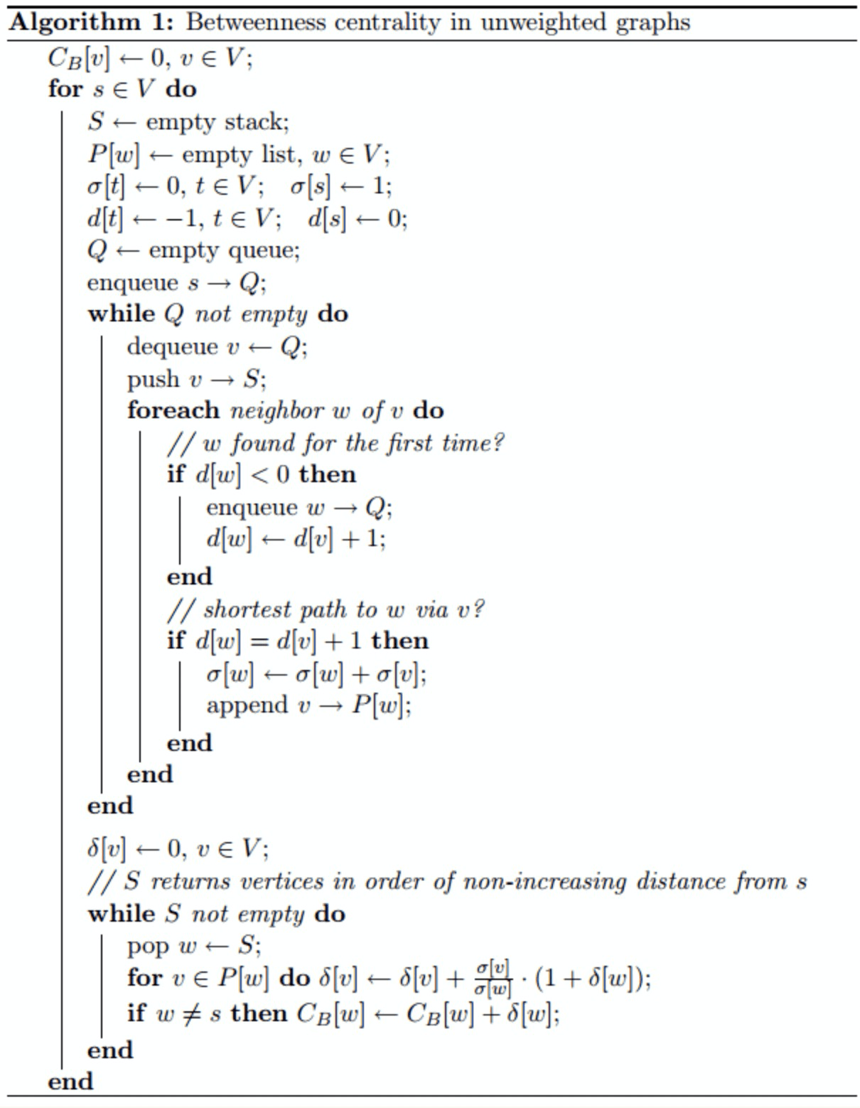
(4) According to the above formula that gets the result of $\delta_{sv}$, the algorithm workflow of Betweenness Centrality in unweighted graphs can be given as follows:

For unweighted graphs, follow the above process.

To calculate the Betweenness Centrality in weighted graphs requires Dijkstra's algorithm, that is, to change the code in the first while loop.

The Betweenness Centrality against NebulaGraph has achieved the algorithms for both weighted and unweighted graphs. For the code, see https://github.com/vesoft-inc/nebula-algorithm/blob/master/nebula-algorithm/src/main/scala/com/vesoft/nebula/algorithm/lib/BetweennessCentralityAlgo.scala.

Computation Examples

Firstly, read the graph data in NebulaGraph to specify the edge data for data reading.

Secondly, make a topological graph based on the edge data of NebulaGraph and perform centrality computation.

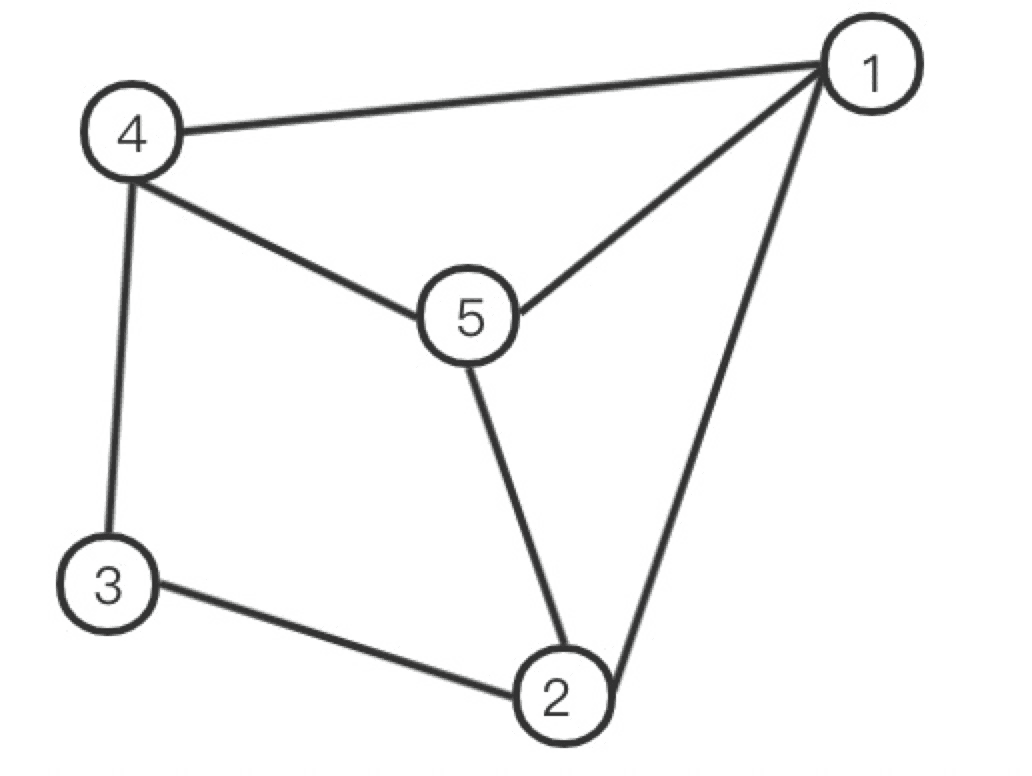
The graph data read in NebulaGraph can be illustrated in the following unweighted graph:

Compute the BC of Vertex 1:

The vertex pair with the shortest path passing through Vertex 1	The total number of shortest paths between the vertex pair	The number of the shortest path passing through Vertex 1
2-4	3 （2-3-4, 2-5-4, 2-1-4）	1
The BC of Vertex 1:	1/3

Compute the BC of Vertex 2:

The vertex pair with the shortest path passing through Vertex 2	The total number of shortest paths between the vertex pair	The number of the shortest path passing through Vertex 2
1-3	2 （1-2-3, 1-4-3）	1
3-5	2（3-2-5, 3-4-5）	1
The BC of Vertex 2:	1

Compute the BC of Vertex 3:

The vertex pair with the shortest path passing through Vertex 3	The total number of shortest paths between the vertex pair	The number of the shortest path passing through Vertex 3
2-4	3 （2-3-4, 2-5-4, 2-1-4）	1
The BC of Vertex 3:	1/3

Compute the BC of Vertex 4:

The vertex pair with the shortest path passing through Vertex 4	The total number of shortest paths between the vertex pair	The number of the shortest path passing through Vertex 4
1-3	2 （1-4-3, 1-2-3）	1
3-5	2（3-4-5, 3-2-5)	1
The BC of Vertex 4:	1

Compute the BC of Vertex 5:

The vertex pair with the shortest path passing through Vertex 5	The total number of shortest paths between the vertex pairs	The number of the shortest path passing through Vertex 5
2-4	3 （2-3-4, 2-5-4, 2-1-4）	1
The BC of Vertex 5:	1/3

Therefore, the BC of each vertex is: Vertex 1: 1/3 Vertex 2: 1 Vertex 3: 1/3 Vertex 4: 1 Vertex 5: 1/3

Result Examples

Data: Read the edge data in the NebulaGraph test, and take srcId, dstId, and rank as the triplet of edges in the topological graph (Source Vertex, Destination Vertex, and Rank).

(root@nebula) [test]> match (v:node) -[e:relation] -> ()  return e
+------------------------------------+
| e                                  |
+------------------------------------+
| [:relation "3"->"4" @1 {col: "f"}] |
+------------------------------------+
| [:relation "2"->"3" @2 {col: "d"}] |
+------------------------------------+
| [:relation "2"->"5" @4 {col: "e"}] |
+------------------------------------+
| [:relation "4"->"5" @2 {col: "g"}] |
+------------------------------------+
| [:relation "1"->"5" @1 {col: "a"}] |
+------------------------------------+
| [:relation "1"->"2" @3 {col: "b"}] |
+------------------------------------+
| [:relation "1"->"4" @5 {col: "c"}] |
+------------------------------------+

Read the edge data in NebulaGraph, set the graph as unweighted, and calculate the Betweenness Centrality of each vertex. The results are as follows:

vid: 4 BC: 1.0
vid: 1 BC: 0.3333333333333333
vid: 3 BC: 0.3333333333333333
vid: 5 BC: 0.3333333333333333
vid: 2 BC: 1.0

Read the edge data of NebulaGraph, set the graph as weighted, and calculate the Betweenness Centrality of each vertex. The results are as follows:

vid: 4 BC: 2.0
vid: 1 BC: 0.5
vid: 3 BC: 1.0
vid: 5 BC: 2.0
vid: 2 BC: 0.0

References

• Paper: A Faster Algorithm for Betweenness Centrality
• The source code of Python's NetworkX realizing Betweenness Centrality: https://github.com/networkx/networkx/blob/master/networkx/algorithms/centrality

Join our Slack channel if you want to discuss with the rest of the NebulaGraph community!