7 Fundamental Use Cases of Social Networks with NebulaGraph Database | EP 2

We have had a thorough introduction to graph data modeling and data import in the application of social network with graph technology.

7 Fundamental Use Cases of Social Networks with NebulaGraph Database | Episode 1

Now, let me introduce more use cases in this episode.

Identifying key people

Identifying influencers in social networks involves using a variety of metrics and methods to identify individuals who have a lot of influence in a given network. This is useful for many business scenarios, such as for marketing or researching the spread of information in a network.

There are many ways to identify them, and the specific methods and information, relationships, and perspectives considered also depend on the type of these key individuals, and the purpose of acquiring them.

Some common methods include looking at the number of followers a person has or the amount of content consumed, their reader engagement on their posts, videos, and the reach of their content (retweets, citations). These methods are also doable on the graph but are rather mundane, so I won't give examples. Here, we can try to derive these key people on the graph using graph algorithms that evaluate and calculate the importance of nodes.

PageRank

PageRank is a very classic graph algorithm that iterates through the number of relationships between points on a graph to get a score (Rank) for each point. It was originally proposed by Google founders Larry Page and Sergey Brin and used in the early Google search engine to sort search results, where Page can be a pun on Larry Page's last name and Web Page.

PageRank has long been abandoned as too simple in modern, complex search engines, but it still shines in other graph-structured web scenarios, where we can roughly assume that all links are of similar importance and run the algorithm to find those key users in social networks.

In NebulaGraph, we can use NebulaGraph Algorithm, NebulaGraph Analytics to run PageRank on large full graphs, while in the daily analysis, validation, and design phases, we don't need to run results on full data, but on very small subgraphs (up to tens of thousands), we can easily run various graph algorithms in the browser to derive methods that can be used for production.

Today, we will use the built-in in-browser graph algorithm function of NebulaGraph Explorer to execute PageRank (the specific method is omitted here, you can refer to the documentation, but it's really just a matter of mouse clicks).

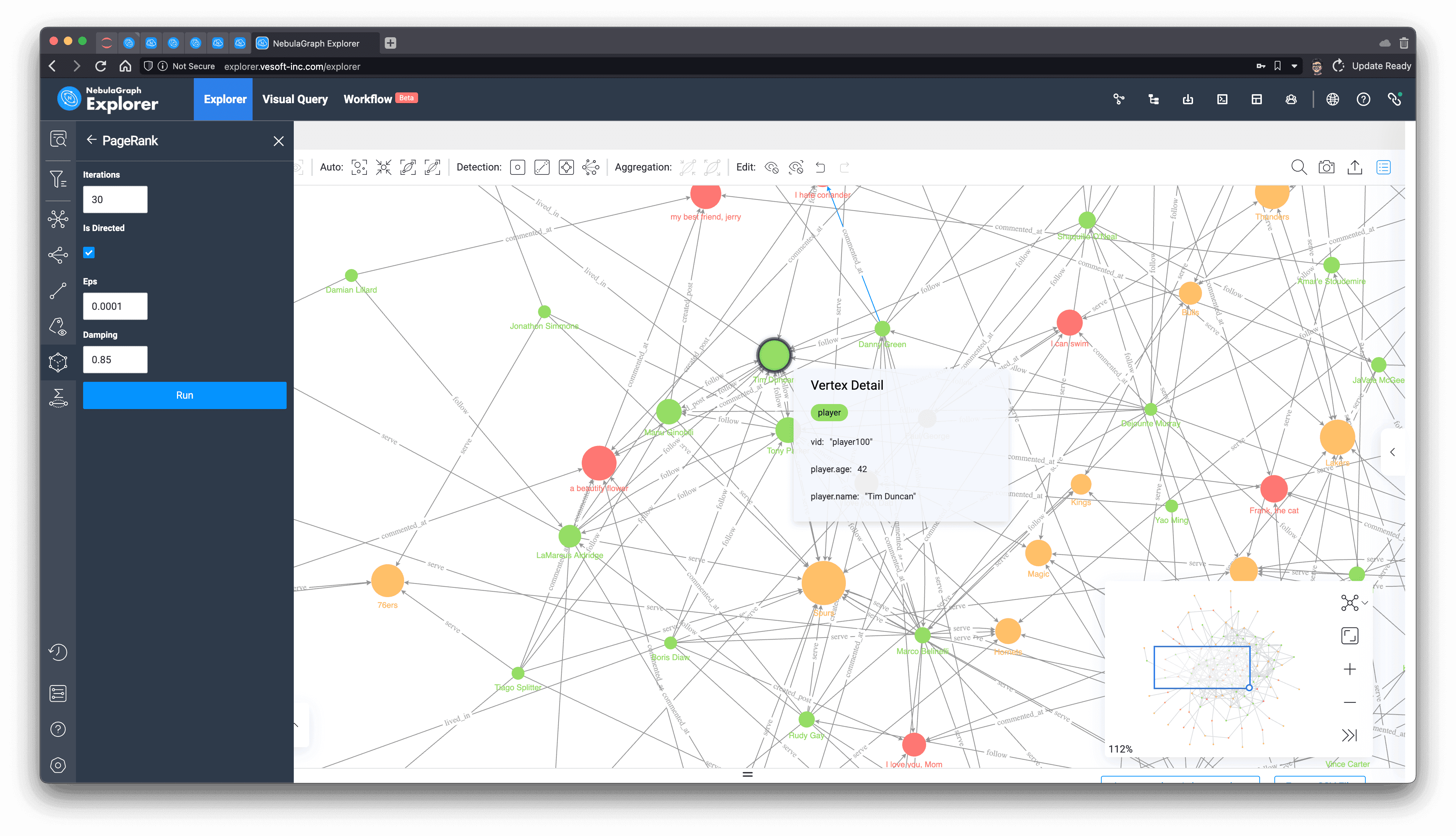
We can see from the above that among all the green players (people) after PageRank calculation, "player.name: Tim Duncan" is the largest one, and the relationship associated with it does seem to be quite a lot, so we select him on the graph, then right-click to invert, select all the points except Tim Duncan, use the backspace key to delete all the other points, and then explore 1 to 5 steps in both directions with him as the starting point. In one step, we get Tim Duncan's subgraph.

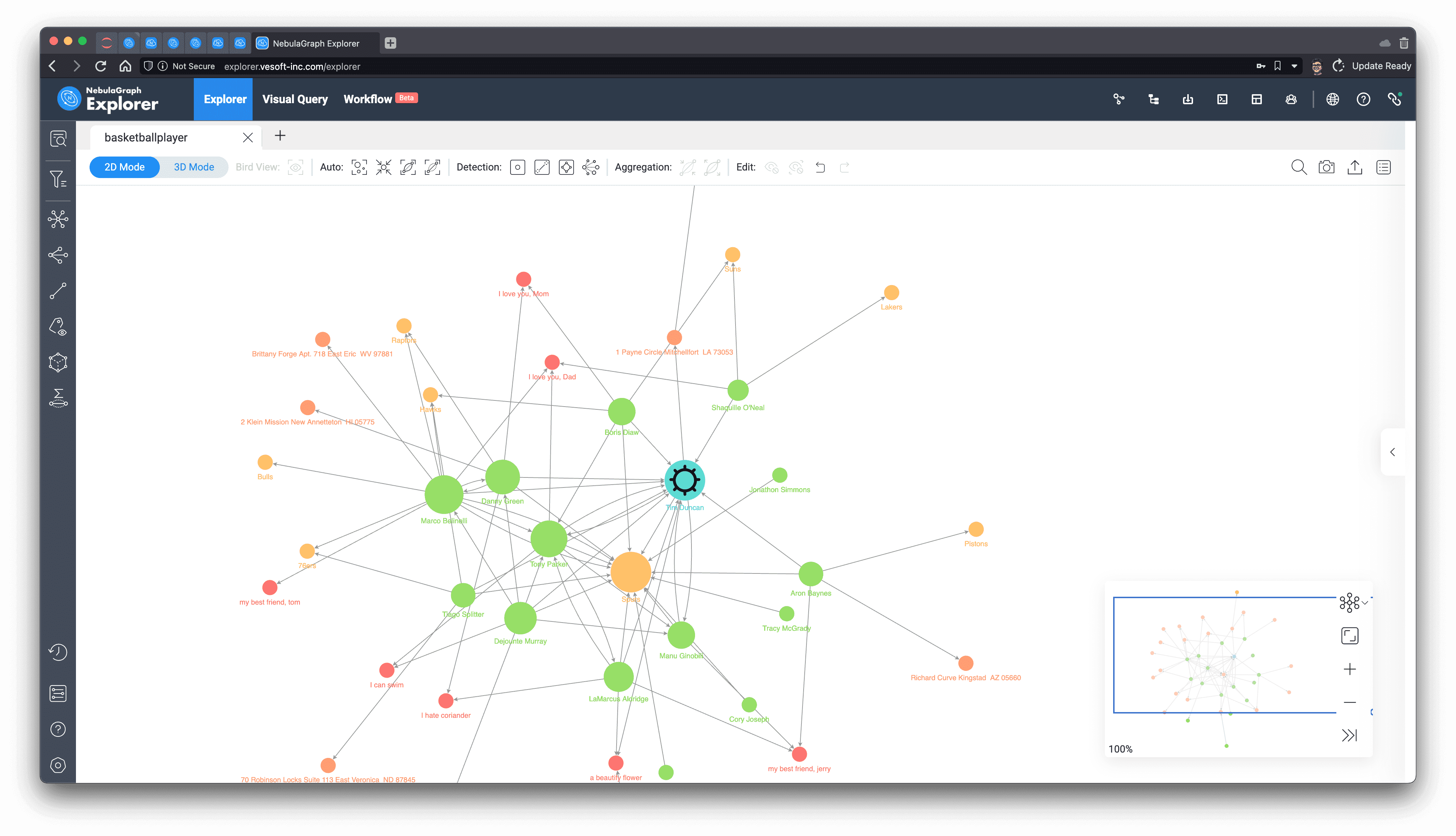
As you can see from the subgraphs, Tim Duncan is associated with a very large number of other players, while some other very popular players have served with him in the very popular Spurs team, which confirms the way PageRank is evaluated.

Now let's see if the algorithm will come to the same conclusion for the other dimensions of determination.

Betweenness Centrality

As you can see from the subgraphs, Tim Duncan is associated with a very large number of other players, while some other very popular players have served with him in the very popular Spurs team, which confirms the way PageRank is evaluated.

Now let's see if the algorithm will come to the same conclusion for the other dimensions of determination.

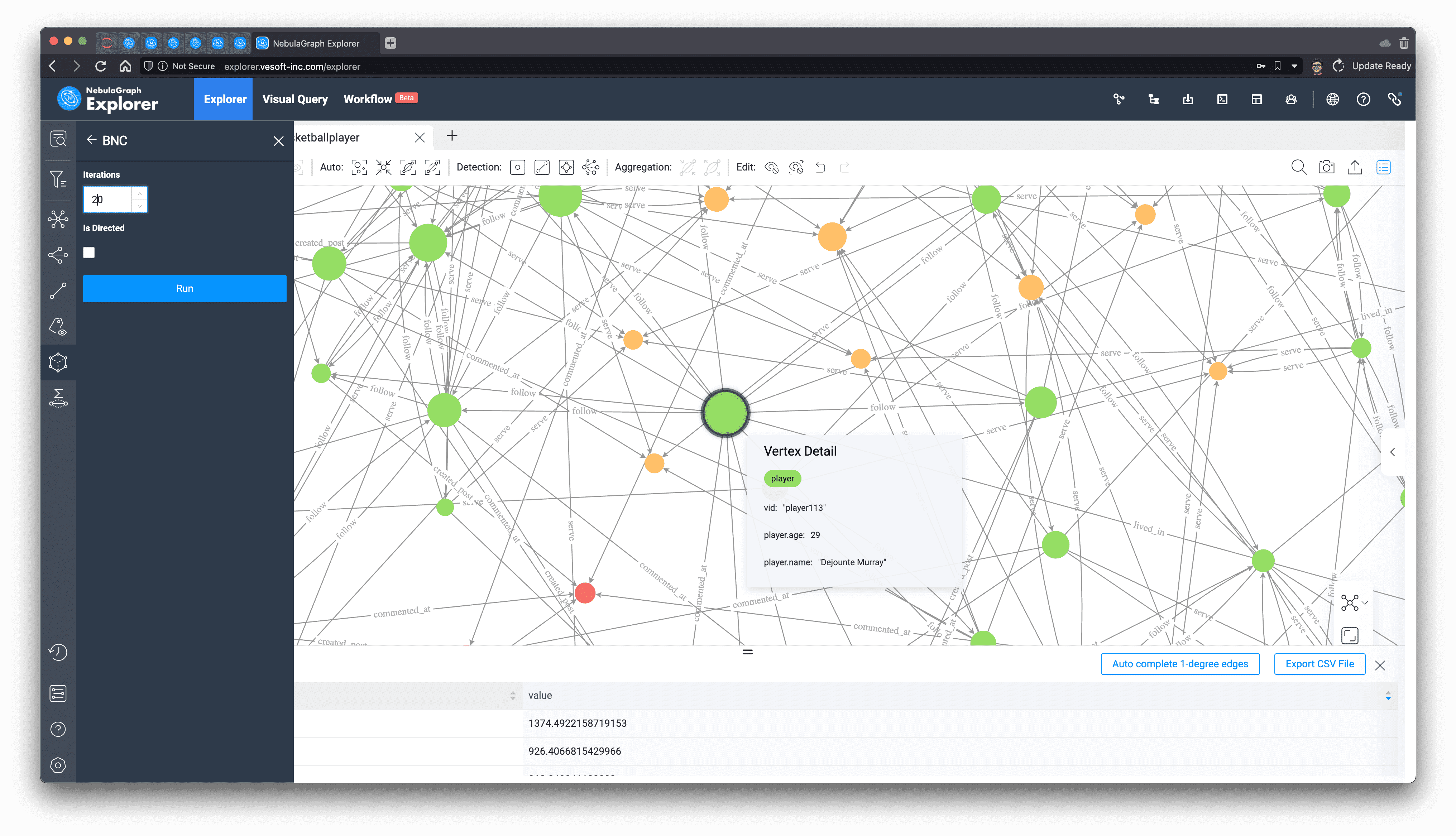
From its five-hop subgraph, it can be seen that unlike the star-shape of the key figure Tim Duncan obtained from PageRank before, Dejounte Murray's subgraph shows clusters, where it is sensory, intuitive to imagine that Dejounte Murray is really on the necessary path of the minimal path between many nodes, while Tim Duncan seems to be associated with more important connecters.

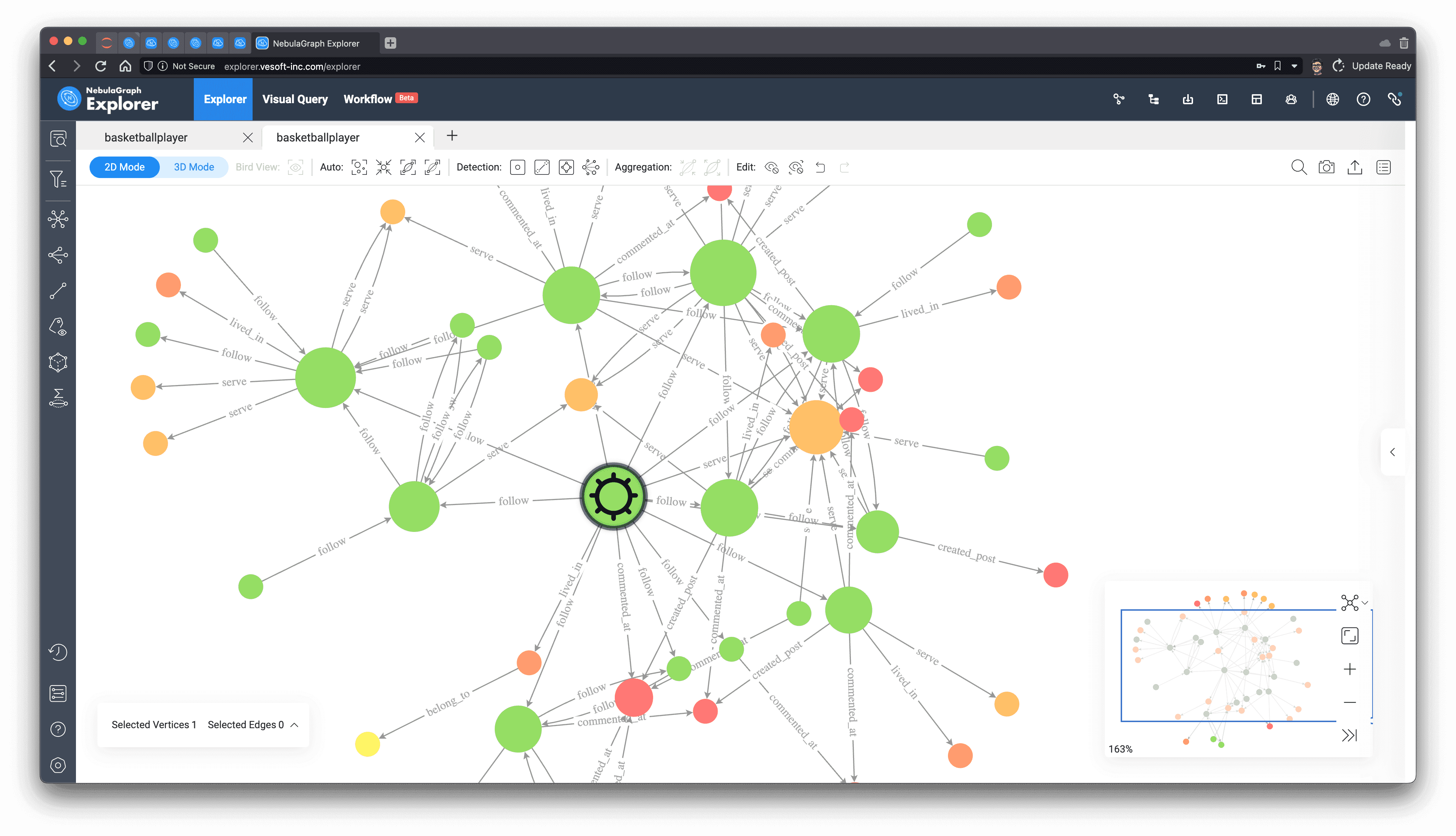
In practical application scenarios, we usually have to understand the definitions in different ways, experiment with different execution results, and analyze to find the structural features that affect the key people we care about, and use them to choose different algorithms for different needs.

Detect communities and clusters

Community detection in social networks is a technique to discover community structure by analyzing social relationships. A community structure is a set of nodes that are closely connected to each other in a social network, graph, and these nodes usually have similar characteristics or interests. For example, a community structure may manifest itself as a group of users who are clustered together based on common topics or interests.

The purpose of community detection is to identify the boundaries of different communities and determine the nodes in each community by analyzing the social network. This process can be done by using various algorithms such as label propagation algorithm, weakly connected component algorithm and Louvain algorithm. By discovering the community structure, we can better understand the structure and characteristics of social networks, and help social network service providers to better infer and predict behaviors in social networks, and help in good social network governance, advertisement placement, marketing, etc.

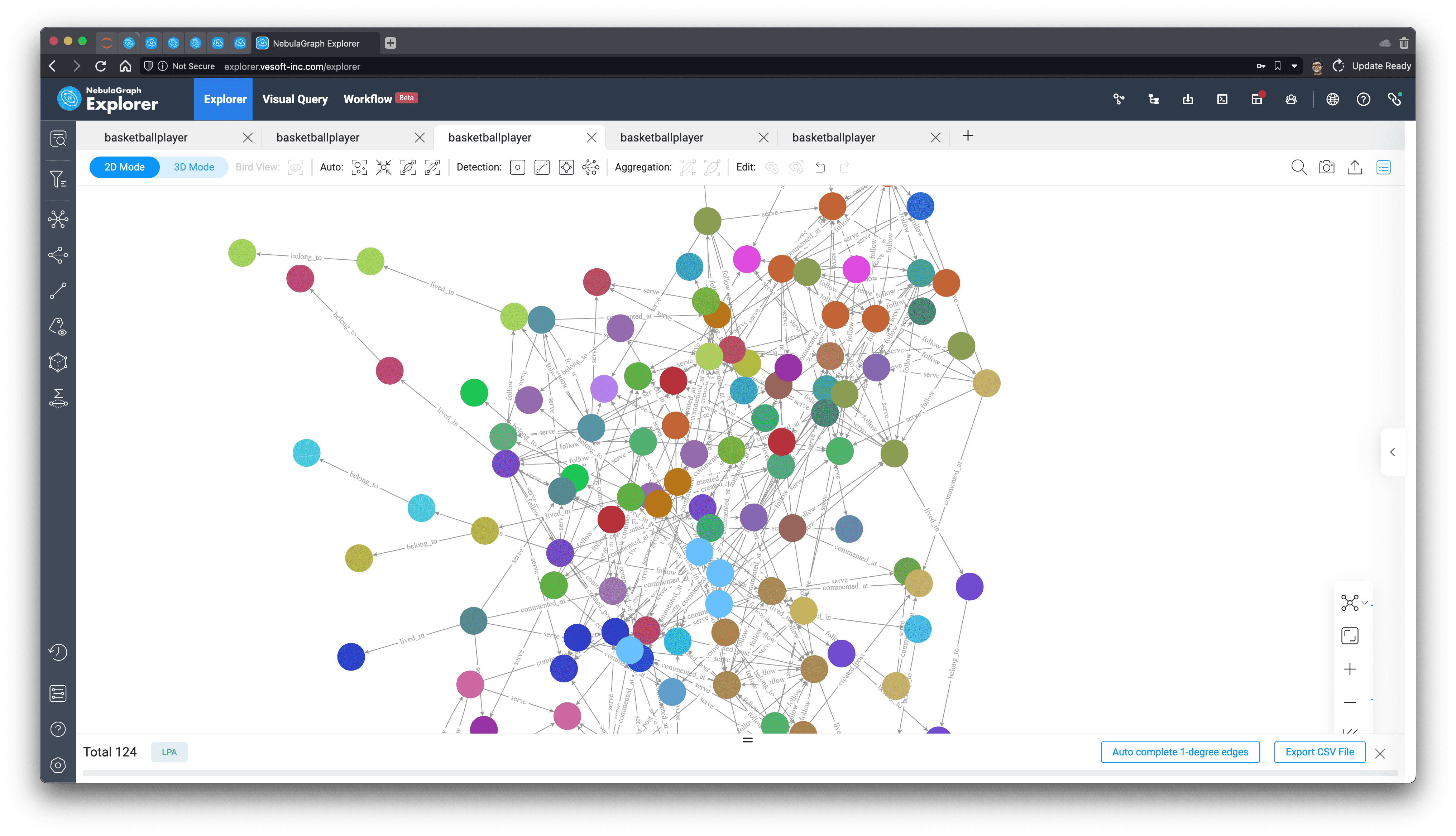
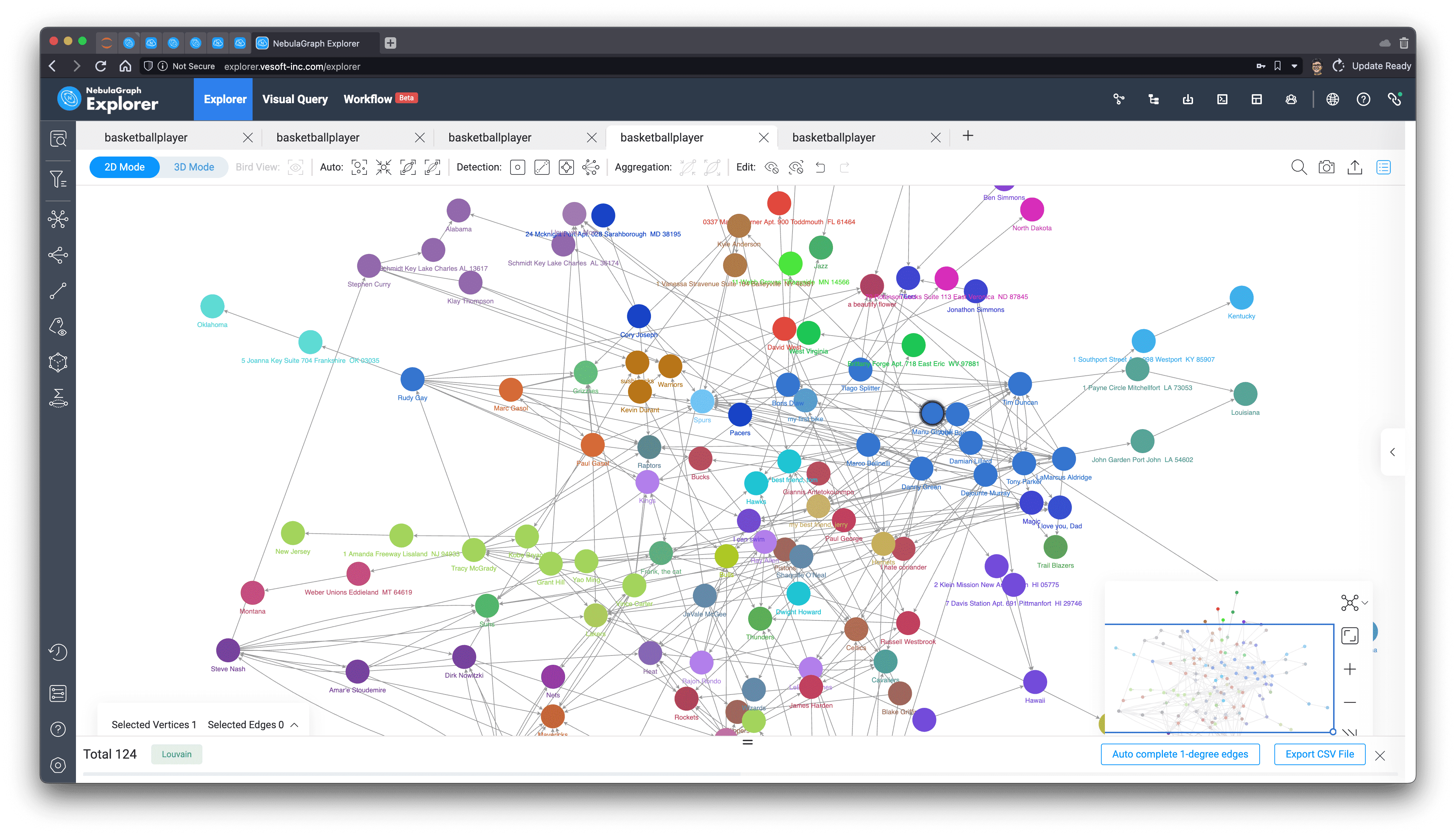
Since our dataset is fake-generated, the results I get under different algorithms do not show the real meaning, so this chapter just shows the results after community identification using several graph algorithms, in real-world cases, we should also use domain knowledge or other technical means on top of that to collaboratively give the portraits and labels of different groups and communities.

Effect of label propagation algorithm.

Louvain algorithm:

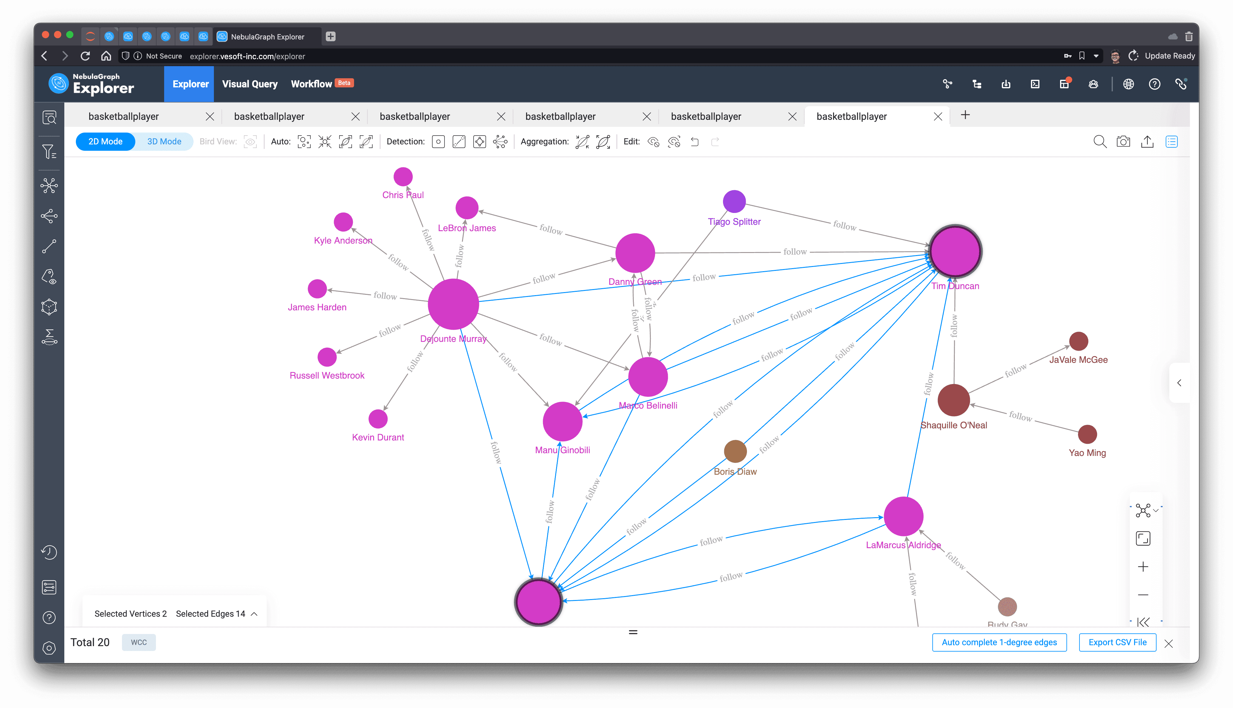
WCC algorithm:

In later sections, we could in better chance verify these algorithms again on smaller and simpler subgraphs, with somewhat more interpretable results.

Friend Closeness

With the community detection algorithm, it is actually possible to obtain friends with similar interests and close associations to some extent, in a global calculation. So how do we get the other close friends of a given user? We can get this information by counting the number of friends this user has in common with him in order to get this information!

Let's take "Tim Duncan" for example, we know that his two-degree friends (friends of friends: (:player{name: "Tim Duncan"})-[:follow]-(f:player)-[:follow]-(fof:player)) are also his friends: Mutual Friend, then it is reasonable to believe that those who have more friends in common with Tim Duncan may have a higher closeness to him.

MATCH (start:`player`{name: "Tim Duncan"})-[:`follow`]-(f:`player`)-[:`follow`]-(fof:`player`),
(start:`player`)-[:`follow`]-(fof:`player`)
RETURN fof.`player`.name, count(DISTINCT f) AS NrOfMutualF ORDER BY NrOfMutualF DESC;

This query shows that "Tony Parker" and Tim have 5 friends in common and are the closest.

fof.player.name	NrOfMutualF
Tony Parker	5
Dejounte Murray	4
Manu Ginobili	3
Marco Belinelli	3
Danny Green	2
Boris Diaw	1
LaMarcus Aldridge	1
Tiago Splitter	1

Here, let's verify this result through visualization!

First, let's see who the common friends (f:) are for each of the friends.

MATCH (start:player{name: "Tim Duncan"})-[:`follow`]-(f:player)-[:`follow`]-(fof:player),
(start:player)-[:`follow`]-(fof:player)
RETURN fof.player.name, collect(DISTINCT f.player.name);

The result:

fof.player.name	collect(distinct f.player.name)
Boris Diaw	["Tony Parker"]
Manu Ginobili	["Dejounte Murray", "Tiago Splitter", "Tony Parker"]
LaMarcus Aldridge	["Tony Parker"]
Tiago Splitter	["Manu Ginobili"]
Tony Parker	["Dejounte Murray", "Boris Diaw", "Manu Ginobili", "Marco Belinelli", "LaMarcus Aldridge"]
Dejounte Murray	["Danny Green", "Tony Parker", "Manu Ginobili", "Marco Belinelli"]
Danny Green	["Dejounte Murray", "Marco Belinelli"]
Marco Belinelli	["Dejounte Murray", "Danny Green", "Tony Parker"]

Then we visualize the result on Explorer.

• First, let's find out all of Tim's 2-degree friend paths

MATCH p=(start:player{name: "Tim Duncan"})-[:`follow`]-(f:player)-[:follow]-(fof:player)
RETURN p

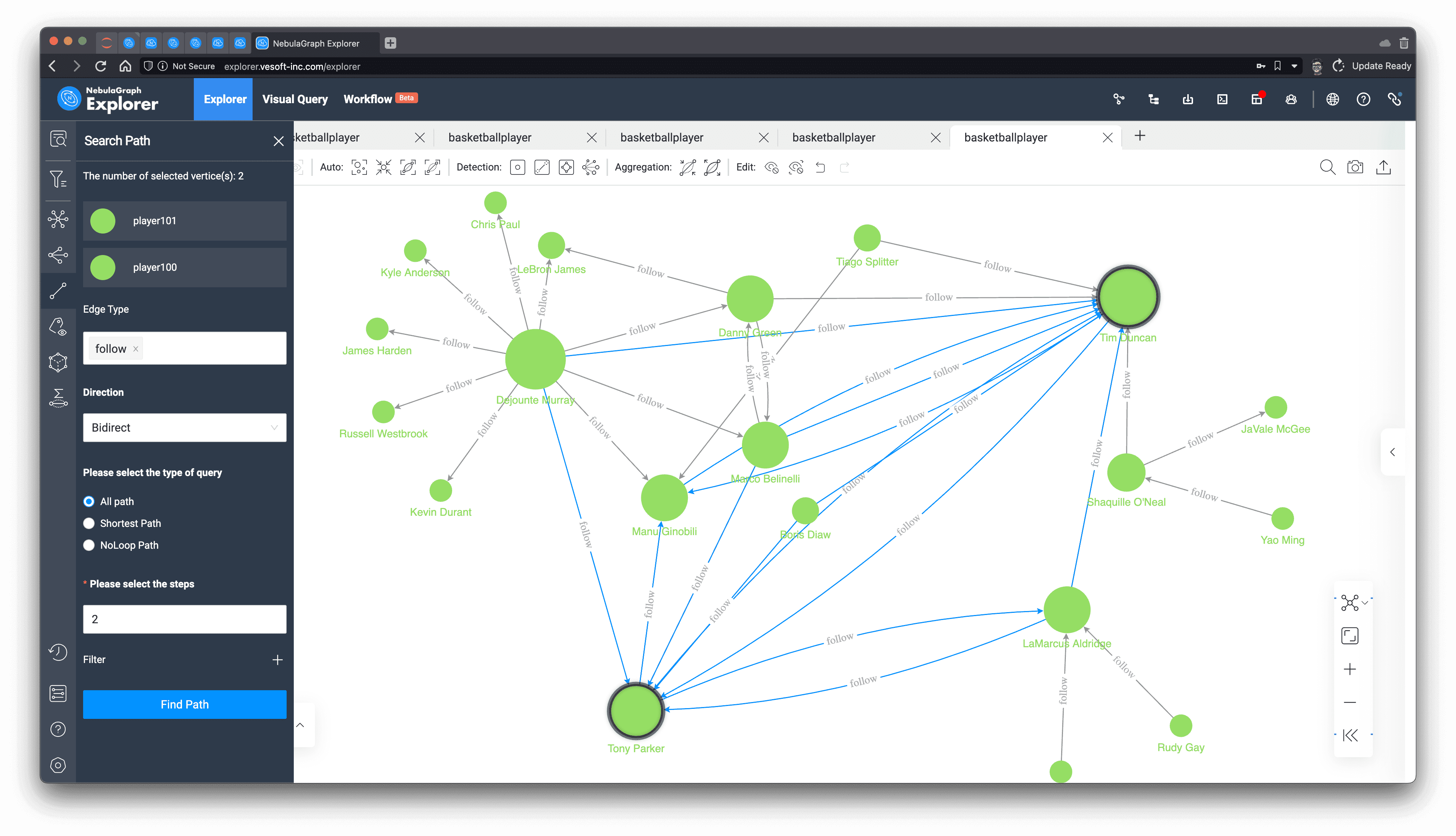
• Then we render the node size by degree in which we select Tim and Tony and find all paths between them for follow type edge, bidirectional, up to 2 hops:

We can see that they are the closest of friends to each other and that their mutual friends are also in the paths.

["Dejounte Murray", "Boris Diaw", "Manu Ginobili", "Marco Belinelli", "LaMarcus Aldridge"]

Small groups in your friends

At this point, as mentioned earlier, the non-authenticity of this dataset itself makes the results of the community discovery algorithm unable to get the insightful connotation of it. Now we can follow this small subgraph to see how groups and communities can be distinguished among Tim's friends.

• Weakly connected components can split Tim's friends into two or three parts that are not connected to each other, which is very much in line with the intuitive understanding and definition of connected components.

• Label propagation, we can control the number of iterations on-demand to delineate different degrees of division by random propagation, which results in a certain degree of differentiation.

  20 iterations

  

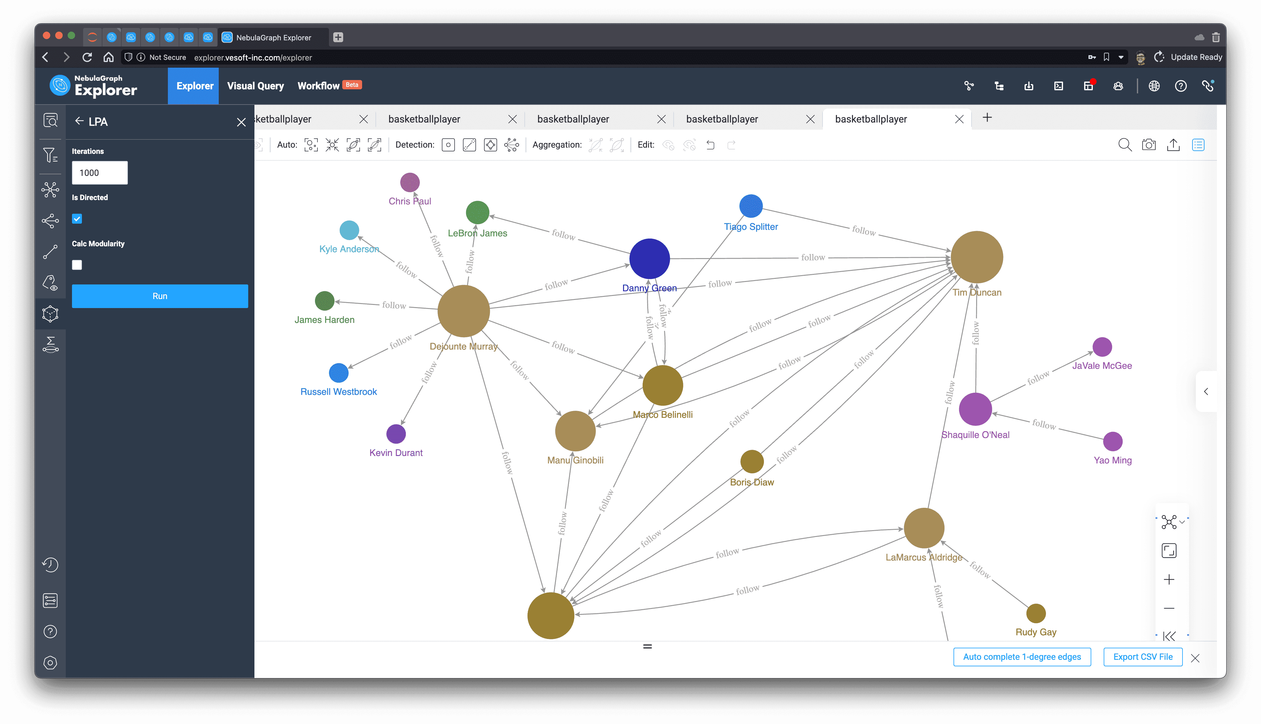
  1000 iterations

  

• Louvain, a more efficient and stable algorithm, basically under this subgraph we can get a very intuitive division with a very small number of iterations.

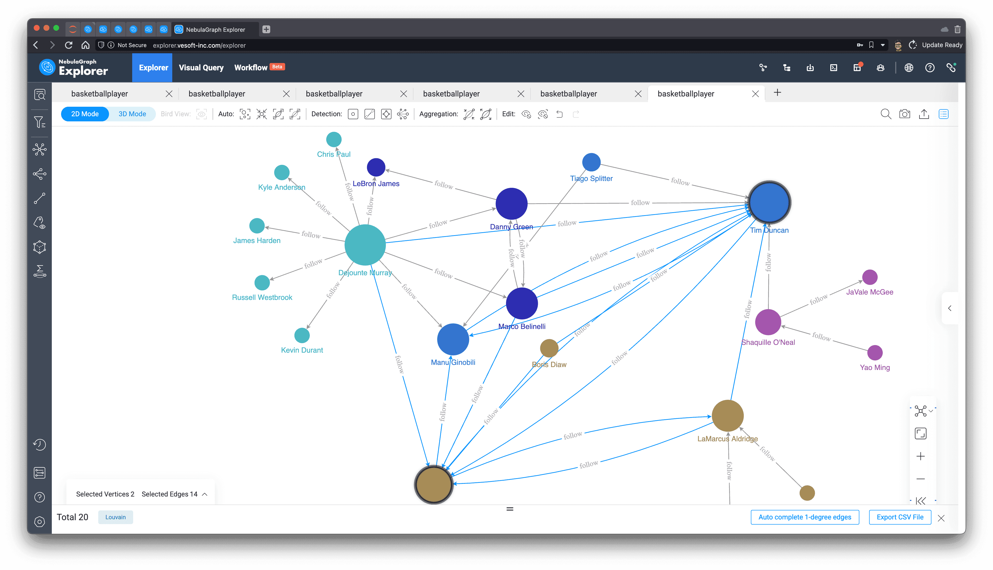
New friend recommendation

Following the previous idea of 2-degree friends (friends of friends), we can easily add those 2-degree friends who are not yet friends as recommended friends, and the sorting rule is the number of friends they have in common with each other:

MATCH (start:player{name: "Tim Duncan"})-[:`follow`]-(f:player)-[:`follow`]-(fof:player)
WHERE NOT (start:player)-[:`follow`]-(fof:player) AND fof != start
RETURN fof.player.name, count(DISTINCT f) AS NrOfMutualF ORDER BY NrOfMutualF DESC;

fof.player.name	NrOfMutualF
LeBron James	2
James Harden	1
Chris Paul	1
Yao Ming	1
Damian Lillard	1
JaVale McGee	1
Kevin Durant	1
Kyle Anderson	1
Rudy Gay	1
Russell Westbrook	1

Obviously, LeBron is the most recommended! And look at who these mutual friends are.

fof.player.name	collect(distinct f.player.name)
James Harden	["Dejounte Murray"]
LeBron James	["Danny Green", "Dejounte Murray"]
Chris Paul	["Dejounte Murray"]
Yao Ming	["Shaquille O'Neal"]
Damian Lillard	["LaMarcus Aldridge"]
JaVale McGee	["Shaquille O'Neal"]
Kevin Durant	["Dejounte Murray"]
Kyle Anderson	["Dejounte Murray"]
Rudy Gay	["LaMarcus Aldridge"]
Russell Westbrook	["Dejounte Murray"]

Again, let's look for LeBron James in the subgraph we just created! And find the two-step, two-way path between them, and sure enough, it only goes through ["Danny Green", "Dejounte Murray"] and, without a direct connection.

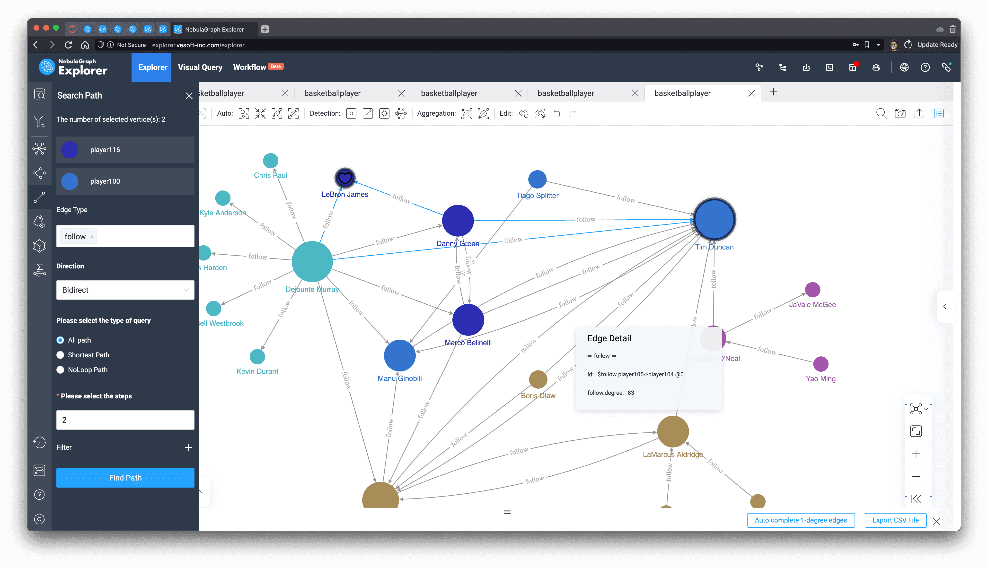
Now, the system could send reminders to both sides: "HEY, maybe you two should make new friends!"

Continue Exploration:

• Pinpointing important content using common neighbors
• Push information flow based on friend relationship and geographic location
• Spatio-temporal relationship mapping